valuation Archives | Page 2 of 2 | ValueScope

950 E. State Highway 114 | Suite 120 | Southlake TX 76092
(817) 481-4995

The Relationship Between S&P 500 Returns, Earnings Growth, P/E Expansion, and Interest Rates

Download the white paper here.

The Relationship Between S&P 500 Returns, Earnings Growth, P/E Expansion, and Interest Rates

The S&P 500 increased from 2,789.80 on January 1, 2018 to 2,924.59 on October 1, 2018, a year-to-date return of 4.83%. As shown in the graph below, this return was fueled by a solid increase in earnings of 9.20% but was partially offset by a contraction of 4.37% in the P/E ratio.

The Relationship Between S&Amp;P 500 Returns, Earnings Growth, P/E Expansion, And Interest Rates

While S&P 500 returns result from both P/E ratio expansion and increases in earnings, these factors have historically been negatively correlated. This means that the offsetting effect that we see above holds for monthly data over a longer period of time. In fact, the relationship for the period January 1970 through October 2018 as determined by linear regression is:

Monthly Increase in Earnings = 0.58% – 27.42% × (Monthly P/E Ratio Expansion)

Based on this regression, a 2% decrease in the P/E Ratio will likely be accompanied by a 1.1% increase in earnings, yielding a negative 0.9% S&P 500 return.

The Relationship Between S&Amp;P 500 Returns, Earnings Growth, P/E Expansion, And Interest Rates

The graph below illustrates the historical relationship of monthly increases in earnings and monthly P/E Ratio expansion.

The Relationship Between S&Amp;P 500 Returns, Earnings Growth, P/E Expansion, And Interest Rates

While we see an offsetting effect in monthly P/E ratio expansion and monthly increases in earnings, both factors have contributed to cumulative S&P 500 returns since January 1970. The index has increased 3,138.4% over this period, while earnings have expanded by 2,037.2% and the P/E ratio has increased by 51.5%.¹ If we allocate the multiplicative component of the S&P 500 to earnings expansion and P/E ratio expansion, we find that 97.5% of the cumulative return in the S&P 500 since January 1970 has come from expansion in earnings, while 2.5% of the cumulative return is attributable to the growth in the P/E ratio. The chart below depicts the cumulative S&P 500 return.

The Relationship Between S&Amp;P 500 Returns, Earnings Growth, P/E Expansion, And Interest Rates

While S&P returns over long periods of time are attributable to earnings expansion, the variation in monthly returns is primarily explained by changes in the P/E ratio (approx. 62%). The chart below illustrates the relationship between monthly S&P 500 returns and the monthly percent change in the P/E ratio.

The Relationship Between S&Amp;P 500 Returns, Earnings Growth, P/E Expansion, And Interest Rates

Historical Distribution of the P/E Ratio

During the period January 1970 to October 2018, the S&P 500 P/E ratio averaged 19.5x. However, for the majority of the period, the P/E ratio was less than the 19.5x average. The P/E ratios had remained above the average for the last 48 months.

During the period January 1987 to October 2018, the P/E ratio averaged 23.5x and the median P/E ratio was 20.5x. In the last 15 years, the average P/E ratio has moved further upwards to 24.5x.

The Relationship Between S&Amp;P 500 Returns, Earnings Growth, P/E Expansion, And Interest Rates

The S&P 500 P/E ratio as of October 1, 2018 was 23.9x, which is 22.6% higher than the historical average of 19.5x. At the same time, it was trading below the last 15 years average of 24.5x.

Interest Rates Compared to P/E Ratio

From our prior paper ² discussing S&P 500 returns, we know that the P/E ratio is theoretically a function of the long-term growth rate in earnings and the required rate of return. From January 1970 to October 2018, the Federal Funds Rate averaged 5.23%. At the same time, the S&P P/E ratio averaged 19.5x. From 1973 until the end of 1991, interest rates were almost always above the historical average. Most notably, in 1980 and 1981, the Federal Funds Rate rose to 20.00% on four occasions over the two-year period, the highest interest rate in United States history. However, the Federal Funds Rate has averaged 3.50% since 1986 and for the last 25 years, interest rates have remained below the historical average, plummeting to 0.15% in 2009. For the following seven years, the interest rate remained low and only began to increase in December of 2015 when the Federal Reserve determined that economic growth had stabilized. Due to low interest rates since the great recession, the Federal Funds Rate has averaged 1.34% in the last 15 years. It can be seen that the average interest rates have been falling for a long time and had only recently picked up. With some recent increases, as of October 2018, the Federal Funds Rate was 2.20%.

The Relationship Between S&Amp;P 500 Returns, Earnings Growth, P/E Expansion, And Interest Rates

It can be observed that the relationship between the P/E ratio and Federal Funds Rate changed during this long period. It appears that the change happened somewhere near 1990. Before August 1987, the P/E ratio and Federal Funds Rate displayed the following logarithmic relationship:

P/E ratio = -6.173 ln (Fed Fund Rate) – 3.6381

The Relationship Between S&Amp;P 500 Returns, Earnings Growth, P/E Expansion, And Interest Rates

Alan Greenspan took over as Fed Chairman in August 1987. He supported an easy money policy and started reducing interest rates soon after. With a change in the Fed’s policy, the relationship between the P/E ratio and interest rates changed to a very weak linear relationship.

P/E ratio = 27.292 – 94.08 (Fed Funds Rate)

The Relationship Between S&Amp;P 500 Returns, Earnings Growth, P/E Expansion, And Interest Rates

The outliers circled above occurred during recessionary periods. After removing the outliers, the relationship between the P/E Ratio and Federal Funds Rate remains weak, as shown in the chart below.

The Relationship Between S&Amp;P 500 Returns, Earnings Growth, P/E Expansion, And Interest Rates

Conclusion

Analysts estimate an 80.7% chance of at least one more increase in the Federal Funds Rate³ before the end of the year. While the prior relationship and financial theory would predict that increasing the Federal Funds Rate would lead to a decline in the P/E ratio through an increase in the required rate of return, our analysis shows that this relationship no longer holds. In future papers, we will investigate the determinants of the S&P 500 required rate of return by examining the implied equity cost of capital.

1. 3,138.4% = (1 + 2,037.2%) x (1 + 51.5%) – 1

2. https://www.valuescopeinc.com/resources/white-papers/the-sp-500-pe-ratio-a-historical-perspective/

3. CME Group, FedWatch Tool, November 8, 2018

The information presented here is not nor should it be treated as investment, financial, or tax advice and is not intended to be used to make investment decisions.

For more information, contact:

The Relationship Between S&Amp;P 500 Returns, Earnings Growth, P/E Expansion, And Interest Rates

Martin Hanan

FOUNDER AND PRESIDENT

Tel: 817-481-4900

mhanan@valuescopeinc.com

Marty Hanan is the founder and President of ValueScope, Inc., a valuation and financial advisory firm that specializes in valuing assets and businesses and in helping business owners in business transactions and estate planning. Mr. Hanan is a Chartered Financial Analyst and has a B.S. Electrical Engineering from the University of Illinois and an MBA from Loyola University of Chicago.

If you liked this blog you may enjoy reading some of our other blogs here.

The Renaissance Board

Download the white paper here.

The Renaissance Board

How to Boost Shareholder Value through Board Mix

Corporate selection of independent board directors has historically followed broad economic and social trends. First came the celebrity board director – CEOs, politicians, and even media stars – who helped increase brand awareness. Then, following Sarbanes-Oxley, came the rise of the audit focused board director who would protect investors from accounting shenanigans. Then, with the digital boom, came the board director with technology expertise who would advise companies on how best to fix and integrate all the IT systems. Most recently, the rise of social media has meant that a marketing and multi-media guru was needed to advise on how to integrate social media into business strategy. Boost Shareholder Value.

Boost Shareholder Value

While it is important to keep up with economic and social trends, it is also important to ensure that the selection criteria for independent board directors matches the underlying goals of the company. We all have heard through the popular press that the primary goal of any corporation is to maximize shareholder wealth, but what is the fundamental responsibility of a board? Simply put, the board exists to protect the interests of the shareholders. The question then is, what is the best way to govern the management and decisions of a company so that shareholder wealth is maximized and protected?

While the component parts to governance (e.g., compensation, audit) are certainly required, effective board governance requires members who can assist management in navigating the maze of value creation strategies, knowing full well that human and financial resources are finite and dynamic. Adding a board member with deep expertise in financial economics and, more specifically, value creation can create a holistic framework from which all decisions can be informed and quantified. Any public or private board that is missing this expertise is likely not optimized, and Management and shareholders are probably not fully served.

So how does a board focused on value creation accomplish these goals? The answer is by concentrating on the variables that most directly impact shareholder wealth: next period cash flow (CF₁) or profits, risk (as measured by the cost of capital (k)), and the growth rate of future cash flow (g).

Boost Shareholder Value

Understanding this formula, we can break the value creation opportunity into its three underlying components.

Path 1 (CF₁): Cash Flow / Profit Maximization: Most organizations are data rich, especially those with numerous transactions. Finding optimal price points and structuring pricing algorithms through elasticity and regression modeling can lead to immense value creation, as every dollar increase in price typically falls to the bottom line. Likewise, unit volume and sales close rates can be increased through similar modeling. This results in revenue and profit growth without significant risk or cost. The increase in profitability results in a substantial increase in value. For example, if you double the profit, you double the value. Optimizing cost structures, especially sales force and executive incentive compensation, can also lead to improved growth and profits.

Real example: I assisted an in-home flooring sales and installation company improve their product pricing and allocation of leads to salespeople by moving from ad hoc processes to algorithms. The company was pricing its product arbitrarily without consideration of all available information, resulting in the company not maximizing its profit. Similarly, leads were not being allocated to salespeople in a manner that optimized close rates and profit. I performed a detailed analysis of all historical transactions for a sample period by SKU to determine the relevant statistics and price variations across product lines. I determined the close rates by salesperson by SKU at varying prices so that we could develop a pricing algorithm that estimated the profit-maximizing price for each SKU based on key characteristics of the transaction. While the optimal stated price increase ranged from 3% to 8% depending on the SKU, the average effective price increase ranged from 1.3% to 4.0% after considering slightly lower close rates. This improved overall gross margin by about 2.5%, which translated to about a 50% increase in net profit and net margin (from about 5% to 7.5%).

Boost Shareholder Value

Path 2 (k): Risk Mitigation and Capital Structure: The weighted average cost of capital is primarily influenced by the market risk, or “systematic” risk, of the firm. However, there are company-specific, or “unsystematic,” risks that influence cash flow and growth as well. Company and shareholder risk can take many forms: lawsuits, price and cost volatility, exogenous variables such as tax and regulation changes, succession, and keyman risk. Many of these shocks can be mitigated through planning and various strategies such as hedging with futures contracts and using long-term employment contracts. Likewise, diversification and counter-cyclical business units can lower both systematic and unsystematic risks. Most common, and often ignored, is succession risk that is both unsystematic and asymmetric (to the downside). Developing long-term incentive plans, carefully crafted employment agreements, and succession plans can greatly lower this risk.

Whatever the cause, meaningful reductions in systematic and/or unsystematic risk often lead to significant and immediate value creation, for both public and private companies. As a result, the overall cost of capital can be minimized, and shareholder value can be enhanced via a more optimal capitalization of the firm.

Real example: I assisted a $1 Billion biofuel production and distribution company with several risk mitigation projects including optimizing its capital structure and developing executive compensation and retention plans. At the time of my analysis, the asset-intensive company was underutilizing debt in its capital structure due to the board’s perceived risks of debt. Utilizing several methodologies, I was able to determine the wealth maximizing capital structure for the widely-held investor group and prove to them that a less conservative approach was more optimal. Furthermore, through cash flow simulation forecasting, I was able to demonstrate and quantify the potential cash flow risks related to taking on additional debt.

In addition to assisting the firm in resolving capital structure issues, I was able to develop an executive compensation program that aligned the interests of management with those of the owners. This plan helped reduce and eliminate the agency issues associated with the non-owner operators and help reduce the unsystematic risk of the firm.

Path 3A (g): Organic Growth: Everyone loves growth. Here’s some simple math about the effect of growth on value: double the expected long-term growth rate from, say, 5% to 10%, and you double the current value. Now, you can see why effectively modeling growth for scale or diversification opportunities, while minimizing execution risk, is vital for any expansion or strategic plan.

Real example: I assisted a fast-casual restaurant chain scale from six to thirty locations by developing an integrated model that allowed the company to project financials on a store-by-store basis, estimate capital expenditures and cash requirements, and project investor and company returns. The model was utilized by the company to develop their organic growth strategy and obtain the required growth capital. The flexibility of the model allowed the company to optimize its capital raise by understanding various scenarios and the resulting returns to each investor.

Path 3B (g): Inorganic Growth: Significant value creation is possible through M&A activity given the proper assessment of price, terms, and strategic fit (i.e. synergy value). Finding, vetting, analyzing, pricing, structuring, and integrating merger partners can change shareholder returns markedly – and quickly. However, M&A can be a double-edged sword. Performed incorrectly, value is destroyed. Additionally, complex ownership structures and derivative securities must be properly analyzed and valued, earnouts need to be effectively constructed, and incentive compensation and roll over equity must be carefully thought through in order for acquisition values to be maximized.

Real example: I assisted a publicly traded industrial packaging products and services company in completing seven acquisitions in two years by developing a valuation model that allowed the firm to better vet potential targets as well as estimate potential synergies and the stock price effect of each deal. As a result, the company grew over the two-year period from $2.8 Billion to $4.2 Billion in revenue, a 22.5% compound annual growth rate.

Conclusion – Value Creation through Board Selection

These all-important decisions and value drivers are critical to creating (or destroying) value for an enterprise and its shareholders. While industry knowledge and specialized expertise are certainly of vital importance, the insight and clarity brought by data and financial analytics should not be compromised. Expertise in analytics, scenario and simulation forecasting, compensation and incentive planning, and financial modeling is key to having an impactful board that can help Management make the right decisions for its shareholders.

For more information, contact:

The Renaissance Board

Martin Hanan

FOUNDER AND PRESIDENT

Tel: 817-481-4900

mhanan@valuescopeinc.com

Marty Hanan is the founder and President of ValueScope, Inc., a valuation and financial advisory firm that specializes in valuing assets and businesses and in helping business owners in business transactions and estate planning. Mr. Hanan is a Chartered Financial Analyst and has a B.S. Electrical Engineering from the University of Illinois and an MBA from Loyola University of Chicago.

If you liked this blog you may enjoy reading some of our other blogs here.

Economic Overview – Third Quarter 2018

U.S. Economic Report – September 30, 2018

Economic Overview – Third Quarter 2018

During the second quarter of 2018, the U.S. economy grew at a feverish 4.2% over the prior quarter. Economic indicators point toward continued economic growth.

Overview of the U.S. Economy

According to the third estimate released by the Bureau of Economic Analysis (BEA), the U.S. economy grew in the second quarter of 2018, with real gross domestic product (GDP) increasing at an annual rate of 4.2%, following a first quarter 2018 increase of 2.2%. The increase in real GDP in the first quarter reflected positive contributions from nonresidential fixed investment, PCE, exports, federal government spending, and state and local government spending that were partly offset by the negative effects from residential fixed investment and private inventory investment.¹ This brings the US economy its seventeenth consecutive quarter with positive GDP growth. For comparison, the longest streak of consecutive quarters is thirty-nine, which occurred between 1991 and 2001.

Forecasters surveyed by the Federal Reserve Bank of Philadelphia predicted, on average, a 3.0% annual real growth rate for the third quarter of 2018 and 2.8% for the fourth. The forecasters predicted, on average, that real GDP will grow 2.8% in 2018, 2.8% in 2019, 1.8% in 2020, and 1.5% in 2021. The forecast for 2019 is higher than previous estimates, while the forecasts for 2020 and 2021 are lower than previous estimates for the same periods.²

Population

Population growth is an important driver of long-term growth in an economy. The total population increased from 326.3 million in August 2017 to 328.6 million in August 2018. The working age population (15-64) increased from 205.6 million in August 2017 to 206.6 million in September 2018. The elderly population (65+) increased from approximately 50.3 million in August 2017 to 50.6 million in August 2018.

The labor force participation rate has not budged in recent years and remains lower than pre-2008 levels. In August 2018, the civilian labor force participation rate was 62.7%. The minimum participation rate in the past decade was 62.3%, recorded in September 2015, while the maximum of 66.4% was recorded in December 2006. This is at least partially explained by the aging population but could be evidence of slack in the labor force.

Employment

Nonfarm payroll employment, according to the Bureau of Labor Statistics (BLS), rose by 201,000 in August 2018. The unemployment rate (U3) in August 2018 was unchanged at 3.9%. The BLS reported job gains in professional and business services, health care, wholesale trade, transportation and warehousing, and mining.³ This is slightly below the Federal Open Market Committee (FOMC) participants’ projections of the long-run natural rate of unemployment, which have a range of 4.0 to 4.6%.

Forecasters surveyed by the Federal Reserve Bank of Philadelphia predicted, on average, that the unemployment rate will be 3.9% in 2018, 3.6% in 2019, 3.7% in 2020, and 4.0% in 2021.⁴

The U6 unemployment rate, which includes all marginally attached workers and those employed part-time for economic reasons, has declined from 8.6% in August 2017 to 7.4% in August 2018. The gap between U3 and U6 has declined from the 10-year high of 7.4% in September 2011 to 3.5% in August 2018.

The average number of weeks unemployed has declined to near pre-2008 levels, to 22.6 weeks in August 2018, from 24.3 in August 2017. This is far below the 10-year high of 40.7 weeks in July 2011, and slightly above the 16.5 weeks in March 2008. The number of jobless claims has also been declining. For the week ending September 22, the number of seasonally adjusted jobless claims was 214,000, while for the prior year that number was 258,000.⁵

Inflation

According to the BLS, inflation, as measured by changes in the Consumer Price Index for All Urban Consumers (CPI-U), increased 0.2% in August 2018 on a seasonally adjusted basis. Over the previous 12 months, the all items index increased 2.7% before seasonal adjustment. The index for all items less food and energy rose 2.2% for the twelve-month period ending August 2018. The energy index rose 10.2% over the last year, while the food index increased 1.4%.⁶ The price pressures measure measures the probability that the personal consumption expenditures price index inflation rate will exceed 2.5% over the next twelve months. This price pressures measure reported a probability of 2.98% in September 2018, which is reasonably low relative to the past five years.⁷

Forecasters surveyed by the Federal Reserve Bank of Philadelphia predicted, on average, headline CPI inflation to be 2.4% in 2018, 2.3% in 2019, and 2.3% in 2020. Over the next ten years, forecasters expect CPI inflation to average 2.20% annually.⁸

Interest Rates

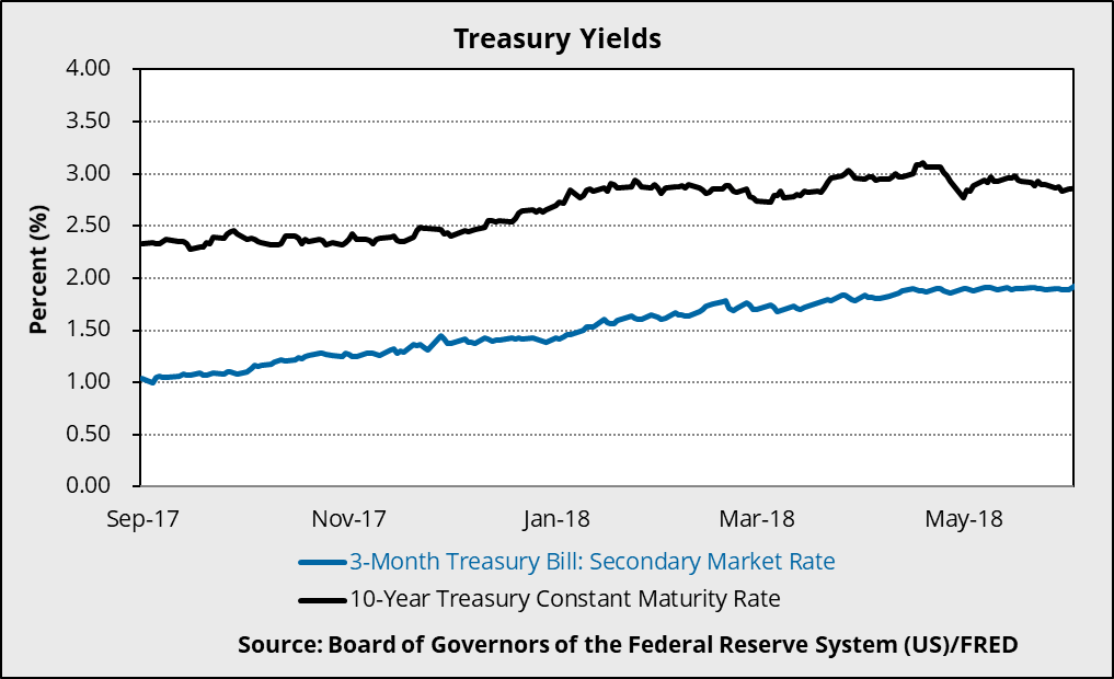
The interest rate on the three-month Treasury bill increased from 1.04% as of September 29, 2017 to 2.15% as of September 28, 2018.⁹ The interest rate on the ten-year Treasury note increased from 2.33% as of September 29, 2017 to 3.05% as of September 28, 2018.¹⁰

On September 26, 2018 the FOMC announced their decision to increase in federal funds target range from 1.75 – 2.0% to 2.0 – 2.25%. This increase was anticipated, and the FOMC also removed the following sentence from their official statement:

The stance of monetary policy remains accommodative, thereby supporting strong labor market conditions and a sustained return to 2 percent inflation.¹¹

The following charts display projections from FOMC officials of the federal funds rate path, as well as the implied projections from federal funds rate futures markets. ^{12, 13}

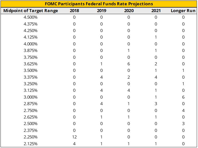
President Trump has expressed concern regarding the FOMC’s decisions to increase rates, and following the September 26, 2018 meeting, he said, “Unfortunately, they just raised interest rates, I am not happy about that.”¹⁴ The following table below represents the market’s reaction during the lead up to and following the FOMC meeting.

As of September 28, 2018, the yields on Moody’s Aaa-rated corporate bonds and Baa-rated corporate bonds were 3.99% and 4.89%, respectively.¹⁵

The spread between the twenty-year and the one-year treasury bills declined from 1.32% as of September 29, 2017 to 0.54% as of September 28, 2018.¹⁶ A combination of increasing short-term interest rates from federal funds rate hikes and tempered long-term growth expectations have caused the yield curve to flatten in recent years. The spread between long- and short-maturity Treasury securities have long been used as a predictive measure for future economic performance. A recent paper from the Federal Reserve showed that the probability of a near-term recession has increased in recent years.¹⁷ However, when additional information was incorporated into their model, such as the excess bond premium,¹⁸ the component of corporate bond spreads in excess of an estimate of the compensation for expected default losses, the recession probability was significantly lower.

Corporate Profits

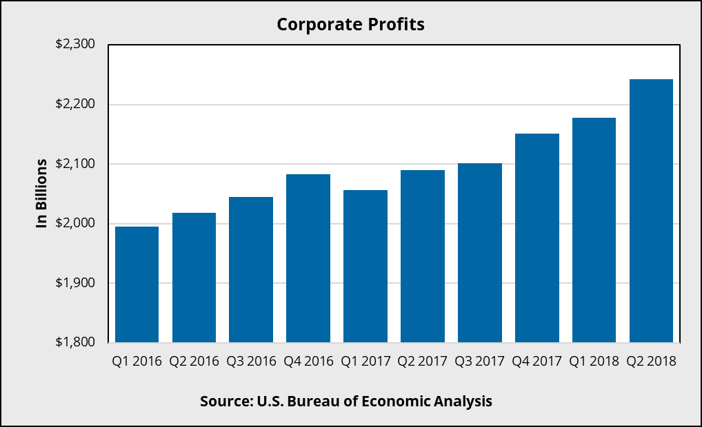
According to the BEA, profits from current production (corporate profits with inventory valuation and capital consumption adjustments) increased $65.0 billion in the second quarter of 2018 over the first, compared to an increase of $26.7 billion in the first quarter of 2018 over the fourth quarter of 2017.¹⁹

Stock Markets

The S&P 500 Total Return²⁰ Index opened at 4,387.96 on September 30, 2017 and closed higher at 5,144.09 on September 30, 2018. This corresponds to an annual return of 17.2%. The Dow Jones Industrial Average Total Return Index opened at 48,051.36 on September 30, 2017 and closed higher at 58,028.52 on September 30, 2018. This corresponds to an annual return of 20.8%. The NASDAQ Composite Total Return Index opened at 7,447.57 on September 30, 2017 and closed higher at 9,322.12 on September 30, 2018.²¹ This corresponds to an annual return of 25.2%. In the graph below, the June 30, 2017 values were set to 100. Each of these indices is near their all-time highs.

Construction & Housing Starts

Construction spending and housing starts are two other important indicators for the economy. Construction spending may indicate the sentiment in real estate markets and the soundness of the economy, while housing starts are an alternative indicator of consumer sentiment. Increases in demand for newly-constructed homes can lead to job growth in the construction industry, increased demand for appliances and furniture, and can have a ripple effect throughout the economy. Housing starts increased from 1,185 thousand units in July 2017 to 1,174 thousand units in July 2018.²² Construction spending, a seasonally adjusted annual rate, increased from $1,242,806 million in July 2017 to $1,315,441 million in July 2018.²³

Consumer Confidence

The Conference Board reported that the Consumer Confidence Index increased in September 2018 to 138.4, up from 134.7 in August 2018.²⁴ The index is based on a survey of consumer perceptions of present economic conditions and expectations of future conditions. The survey is based on a representative sample of 5,000 U.S. households and is considered a leading indicator of future consumer expenditures and economic activity.

The University of Michigan Survey of Consumers reported that the Index of Consumer Sentiment increased in September 2018 to 100.1, up from 96.2 in August 2018 and 95.1 in September 2017.²⁵ The index is based on a survey of consumer perceptions of present economic conditions and expectations of future conditions. The survey is based on a sample of 500 phone interviews consisting of 50 core questions are conducted across the continental U.S. This is considered a leading indicator of future consumer expenditures and economic activity.

According to Surveys of Consumers chief economist, Richard Curtin, the primary driver for the September gain was among households with incomes in the bottom third, whose index value was the highest since November 2000. On the contrary, the index for households with incomes in the top third fell 8.1% during the past seven months. Concerns over the negative impacts of tariffs were cited by nearly one-third of all consumers in September.

Conclusion

In conclusion, the economy continued to perform well in the second quarter of 2018. Economic growth exceeded expectations, reaching over 4% annualized growth for the first time since quarter three of 2014. Inflation has been modest while unemployment remains low, hovering around FOMC participants’ projections of the natural rate of unemployment. Equities markets have been performing exceptionally well, near all-time highs, and both consumer and investor sentiment remains optimistic. Threats to the economy include potential ramifications from rising tariffs, the impact of the Federal Reserve’s decision to increase the federal funds rate, and political instability as we approach the midterm elections.

The following table displays a summary of the economic indicators, their performance over the past year, and whether this is viewed as a positive or negative sign for the economy at large. The leading, lagging, and coincident indices were obtained from The Conference Board.

1. U.S. Department of Commerce, Bureau of Economic Analysis, Gross Domestic Product: Second Quarter 2018 (Third Estimate), September 27, 2018

2. Federal Reserve Bank of Philadelphia, Third Quarter 2018 Survey of Professional Forecasters, August 10, 2018

3. United States Department of Labor, Bureau of Labor Statistics, The Employment Situation: August 2018, September 7, 2018

4. Federal Reserve Bank of Philadelphia, Second Quarter 2018 Survey of Professional Forecasters, August 10, 2018

5. United States Department of Labor, Bureau of Labor Statistics, Unemployment Insurance Weekly Claims, September 27, 2018

6. United States Department of Labor, Bureau of Labor Statistics, Consumer Price Index: August 2018, September 13, 2018

7. Federal Reserve Bank of St. Louis, Federal Reserve Economic Data, Series: STLPPM, Price Pressures Measure, last accessed October 1, 2018

8. Federal Reserve Bank of Philadelphia, Third Quarter 2018 Survey of Professional Forecasters, August 10, 2018

9. Federal Reserve Bank of St. Louis, Federal Reserve Economic Data, Series: DTB3MS, 3-Month Treasury Bill: Secondary Market Rate, last accessed October 1, 2018

10. Federal Reserve Bank of St. Louis, Federal Reserve Economic Data, Series: DGS10, 10-Year Treasury Constant Maturity Rate, last accessed October 1, 2018

11. Wall Street Journal, Fed Statement Tracker, https://projects.wsj.com/fed-statement-tracker-embed/

12. Federal Open Market Committee, Summary of Economic Projections, September 26, 2018

13. Federal Reserve Bank of Atlanta, Market Probability Tracker, last accessed September 27, 2018

14. USA Today, “Why Trump’s Fed-bashing is bad for the economy,” September 26, 2018

15. Federal Reserve Bank of St. Louis, Federal Reserve Economic Data, Series: DAAA, Moody’s Seasoned Aaa Corporate Bond Yield©, Series: DBAA, Moody’s Seasoned Baa Corporate Bond Yield©, last accessed October 1, 2018

16. U.S. Department of the Treasury, Daily Treasury Yield Curve Rates, last accessed October 1, 2018

17. Johansson, Peter, and Andrew Meldrum (2018). “Predicting Recession Probabilities Using the Slope of the Yield Curve,” FEDS Notes. Washington: Board of Governors of the Federal Reserve System, March 1, 2018, https://doi.org/10.17016/2380-7172.2146

18. Gilchrist, S., and E. Zakrajšek (2012), “Credit Spreads and Business Cycle Fluctuations,” American Economic Review 102(4), pp. 1692-1720

19. U.S. Department of Commerce, Bureau of Economic Analysis, Corporate Profits: Second Quarter 2018, September 27, 2018

20. Total return indices include returns from both income and capital gains

21. S&P Capital IQ Database, last accessed October 1, 2018

22. Federal Reserve Bank of St. Louis, Federal Reserve Economic Data, Series: HOUST, Housing Starts, last accessed October 1, 2018

23. Federal Reserve Bank of St. Louis, Federal Reserve Economic Data, Series: TTLCONS, Total Construction Spending, Seasonally Adjusted Annual Rate, last accessed October 1, 2018

24. The Conference Board, Consumer Confidence Index, September 25, 2018

25. University of Michigan, Surveys of Consumers, September 2018

For more information, contact:

Economic Overview - Third Quarter 2018

Martin Hanan

FOUNDER AND PRESIDENT

Tel: 817-481-4900

mhanan@valuescopeinc.com

Marty Hanan is the founder and President of ValueScope, Inc., a valuation and financial advisory firm that specializes in valuing assets and businesses and in helping business owners in business transactions and estate planning. Mr. Hanan is a Chartered Financial Analyst and has a B.S. Electrical Engineering from the University of Illinois and an MBA from Loyola University of Chicago.

If you liked this blog you may enjoy reading some of our other blogs here.

Economic Overview – First Quarter 2018

Overview of the U.S. Economy

Economic Overview – First Quarter 2018

According to the third estimate released by the Bureau of Economic Analysis (BEA), the U.S. economy grew in the fourth quarter of 2017, with real gross domestic product (GDP) increasing at an annual rate of 2.9%, following a third quarter increase of 3.2%. The increase in real GDP in the fourth quarter reflected positive contributions from personal consumption expenditures, nonresidential fixed investment, exports, residential fixed investment, state and local government spending, and federal government spending that were partly offset by a negative contribution from private inventory investment.

Forecasters surveyed by the Federal Reserve Bank of Philadelphia predicted, on average, a 3.0% annual real growth rate for the first quarter of 2018 and 2.9% for the second quarter of 2018. The forecasters predicted, on average, that real GDP will grow 2.8% in 2018, 2.5% in 2019, 2.0% in 2020, and 1.7% in 2021. The forecasts for 2018, 2019, and 2020 are higher than previous estimates for the same periods.

Employment

Nonfarm payroll employment, according to the Bureau of Labor Statistics (BLS), rose by 313,000 in February 2018. The unemployment rate in February 2018 was 4.1%. The BLS reported job gains in construction, retail trade, professional and business services, manufacturing, financial activities, and mining.

Forecasters surveyed by the Federal Reserve Bank of Philadelphia predicted, on average, that the unemployment rate will be 4.0% in 2018, 3.8% in 2019, 3.9% in 2020, and 4.0% in 2021.

Inflation

According to the BLS, inflation, as measured by changes in the Consumer Price Index for All Urban Consumers (CPI-U), increased 0.2% in February 2018 on a seasonally adjusted basis. Over the previous 12 months, the all items index increased 2.2% before seasonal adjustment. The index for all items less food and energy rose 1.8% for the twelve-month period ending January 2018. The energy index rose 7.7% over the last year, while the food index increased 1.4%. Forecasters surveyed by the Federal Reserve Bank of Philadelphia predicted, on average, inflation is expected to be 2.1% in 2018, 2.2% in 2019, and 2.3% in 2020. Over the next ten years, forecasters expect CPI inflation to average 2.25% annually.

Interest Rates

The interest rate on the three-month Treasury bill increased from 0.75% as of March 31, 2017 to 1.70% as of March 31, 2018. The interest rate on the ten-year Treasury note increased from 2.40% as of March 31, 2017 to 2.74% as of March 31, 2018.

As of March 31, 2018, the yields on Moody’s Aaa-rated corporate bonds and Baa-rated corporate bonds were 3.77% and 4.59%, respectively.

Yield Curve

The spread between the thirty-year and the one-year treasury bills declined from 1.99% as of March 31, 2017 to 0.88% as of March 31, 2018.

Economic Overview - First Quarter 2018

Corporate Profits

According to the BEA, profits from current production (corporate profits with inventory valuation and capital consumption adjustments) decreased $1.1 billion in the fourth quarter over the third, in contrast to an increase of $90.2 billion in the third quarter over the second quarter.

Stock Markets

The S&P 500 Total Return Index opened at 4,086.29 on March 31, 2017 and closed higher at 4,630.64 on March 31, 2018. This corresponds to an annual return of 13.3%. The NASDAQ Composite Total Return Index opened at 6,741.02 on March 31, 2017 and closed higher at 8,140.57 on March 31, 2018. This corresponds to an annual return of 20.8%. The Dow Jones Industrial Average Total Return Index opened at 43,779.79 on March 31, 2017 and closed higher at 52,270.30 on March 31, 2018. This corresponds to an annual return of 19.4%. In the graph below, the March 31, 2017 values were set to 100.

Consumer Confidence

The Conference Board reported that the Consumer Confidence Index decreased in March 2018 to 127.7, down from 130.0 in February 2018.The index is based on a survey of consumer perceptions of present economic conditions and expectations of future conditions. The survey is based on a representative sample of 5,000 U.S. households and is considered a leading indicator of future consumer expenditures and economic activity.

The University of Michigan Survey of Consumers reported that the Index of Consumer Sentiment increased in March 2018 to 101.4, up from 99.7 in February 2018 and 96.9 in March 2017. The index is based on a survey of consumer perceptions of present economic conditions and expectations of future conditions. The survey is based on a sample of 500 phone interviews consisting of 50 core questions are conducted across the continental U.S. This is considered a leading indicator of future consumer expenditures and economic activity.

For more information, contact:

Economic Overview - First Quarter 2018

Martin Hanan

FOUNDER AND PRESIDENT

Tel: 817-481-4900

mhanan@valuescopeinc.com

Marty Hanan is the founder and President of ValueScope, Inc., a valuation and financial advisory firm that specializes in valuing assets and businesses and in helping business owners in business transactions and estate planning. Mr. Hanan is a Chartered Financial Analyst and has a B.S. Electrical Engineering from the University of Illinois and an MBA from Loyola University of Chicago.

If you liked this blog you may enjoy reading some of our other blogs here.

Ten Reasons to Get a Business Valuation Prior to a Transaction!

Top Ten Reasons to get a Valuation

Business owners and shareholders cannot adequately plan for a sale or merger unless they understand the price that the business will bring in a fair transaction. In order to know this price, an appropriate valuation is required.

The right valuation will:

Clearly indicate the value and value drivers of the business, arming sellers with the tools necessary to negotiate the best possible price.
Identify how to support a higher value prior to the sale by adjusting for related-party transactions and/or expenses (e.g., owners’ compensation, related-party leases, and other perks).
Help determine the optimal time for a sale by gaining an understanding of general M&A trends and specific trends in your industry.
Show expected future wealth and returns under multiple scenarios: hold for now, sell all or some, recapitalize with debt or new equity partners, bring in a strategic partner, invest new capital for growth, etc.
Help with retirement planning by structuring a transaction to minimize estate taxes.
Help determine optimal transaction terms, lowering risk and improving returns.
Show you how your business compares to your peers. This will help identify areas to increase the value of the business.
Show the “intrinsic value” of the business under current ownership and the “fair market value” of the business to others.
Assess and demonstrate synergies to a specific-buyer, supporting that they could pay a price above the fair market value, and still earn above-market expected returns.
Help identify the segments of your business that are most valuable, allowing management to focus on those areas that will most impact the overall business’ value.

For more information, contact:

Ten Reasons To Get A Business Valuation Prior To A Transaction!

Martin Hanan

FOUNDER AND PRESIDENT

Tel: 817-481-4900

mhanan@valuescopeinc.com

Marty Hanan is the founder and President of ValueScope, Inc., a valuation and financial advisory firm that specializes in valuing assets and businesses and in helping business owners in business transactions and estate planning. Mr. Hanan is a Chartered Financial Analyst and has a B.S. Electrical Engineering from the University of Illinois and an MBA from Loyola University of Chicago.

If you liked this blog you may enjoy reading some of our other blogs here.

Pitfalls of Using Life Settlement Transactions to Value Split-Dollar Loan Receivables

Using Life Settlement Transactions to Value Split-Dollar Loan Receivables

Large Estates

For large estates which often plan on using life insurance with large premiums to reduce the value of the estate, split-dollar life insurance offers an attractive method for funding the premiums with favorable gifting consequences. However, the IRS has begun cracking down on the valuation of the split-dollar loan receivables transferred by the loan holders. One of the primary issues has been the use of life settlement transactions to determine the value of the split-dollar loan receivables for gift or estate tax purposes.

Characteristics of Life Settlements

The characteristics of life settlements and split-dollar loan receivables are not similar; therefore, they are not comparable. Using life settlement transactions as a basis for determining the discount rate to apply to split dollar loan receivables inflates the discount rate, which in turn undervalues the receivable. Life settlements include more risk factors and greater underwriting, transaction, and oversight costs than split dollar loan receivables; therefore, life settlements require a higher rate of return/discount rate. The figure below summarizes the risk characteristics of the Life Settlement industry:[1]

Using Life Settlement Transactions To Value Split-Dollar Loan Receivables

Life Expectancy

Life expectancy and modeling error is less significant for healthy, long–lived policies, as is typical with split-dollar loan receivables. The main risk in the Life Settlement industry involves life expectancy estimation.[2] The underestimation of life expectancies for Life Settlements could possibly lead to losses, due to the ongoing premium payments not present with split-dollar loan receivables. Statistically, the probability that an individual will live longer than their life expectancy is 50%.[3] To make up for this, life insurance policies that are purchased in the Life Settlement market are typically for insureds with health impairments, and with a higher discount rate.

In a study performed on open-end funds in U.S. Life Settlements, the realized returns found for 2003 to 2010 were 4.9%.[4] During the same period, the London Business School Study calculated expected IRRs ranging from 11.0% to 18.8%.[5] The risks associated with Life Settlements, and specifically with life expectancy estimates, cause realized returns to be much less than expected returns.

[1] Perera, Nemo and Brian Reeves, Risk Mitigation for Life Settlements, The Journal of Structured Finance, Summer 2006, p. 56

[2] Januario, Alfonso V. and Narayan Y. Naik, Testing for Adverse Selection in Life Settlements: The Secondary Market for Life Insurance Policies, London Business School, July 23, 2014, p. 7

[3] Perera p. 59

[4] Braun, Alexander, Nadine Gatzert and Hato Schmeiser, Performance and Risks of Open-End Life Settlement Funds, Journal of Risk and Insurance 79, pp. 193-229

[5] Januario p. 23

Pitfalls Of Using Life Settlement Transactions To Value Split-Dollar Loan Receivables

Michael Conroy, CFA

DIRECTOR

Tel: 817-481-6348

mconroy@valuescopeinc.com

Mr. Conroy has more than 20 years of consulting and business valuation experience, concentrating on complex estate and gift valuation matters. He provides business valuation and financial consulting services to companies in a broad range of industries. Working with domestic and international clients, Mr. Conroy has performed thousands of business appraisals involving gift and estate tax, financial reporting, mergers, and acquisitions (valuations for buyers/sellers, fairness, and solvency opinions), litigation support, expert testimony, and other company requirements (including stock options and ESOPs). Mr. Conroy previously worked with the national valuation firm CBIZ Valuation Group, LLC here he was a senior manager. Prior to that, he taught chemistry and physics to high school and college students at Xavier College in Ba, Fiji, for two years as a U.S. Peace Corps volunteer.